Ep 17 – Multi-Compartmental Model – Part One: Half-Life, Time Constant and Bi-Exponential Decay
8 January 2025
Contents
This FRCA podcast series will cover the multi-compartmental model
We shall cover half-time, time constant, natural logs, Bi-Exponential Decay and Ficks Law of Diffusion. This is the build up to compartmentalising humans for TCI – these compartments are distinct but not necessarily anatomic or truly, physiologically defined elements, they are pharmaceutically convenient divisions of a human.
Half-Life aka t1/2 (Gordon Freeman is no where to be seen)
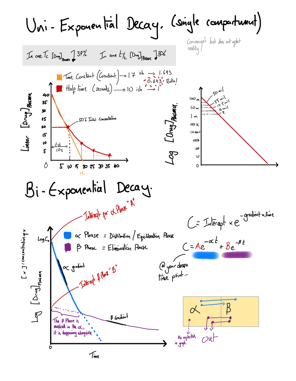
Half-life is the time required for the plasma concentration of a drug to reduce by half, influencing dosing intervals and duration of drug action. Describes the time it is taken for an amount of substance to halve in its amount. Can apply to the decay of radioactive substances, or the reduction of plasma concentration of drug.
It can be derived in a number of ways, either by considering its clearance against its plasma availability (ie if it is a mostly plasma oriented molecule its clearance will differ than something that its very lipid soluble.)
Half lives – are introduced thinking about it in a single compartment flavour but also applies to ‘decay constants / clearance constants in multi compartmental pharmacological models’
Time Constant, Tc. Tau (t)
The time constant (τ) is the time for plasma concentration to reach zero if the initial rate of decline continued; numerically, τ = 1/k and equals 1.44 × t½.
Time Constant is the time it would take for a plasma concentration of a drug to fall to zero if the initial decay rate continued (i.e. if it was a fixed rate of decay) The unit is time.
Single-Compartment Kinetics: Key Formulae
The single-compartment model yields three linked equations: half-life = 0.693/k, time constant = 1/k, and clearance = Volume of Distribution × k.
Time constant and half life are associated by a number, 0.693.
This number also crops up when thinking about natural logs natural log (2) – 0.693
-
Half life = 0.693 * Time constant (Thanks Ben!)
-
Half life = 0.693 / k
-
Half life = 0.693 x VD / clearance
-
Time constant is the inverse of the rate constant of elimination (K)
-
Time constant = 1/k
-
Time constant = 0.693 / half-life
4-5 half times or 3 time constants to reach steady state.
Remember
K = Rate constant for elimination (aka K the fraction of a substance removed per unit time)
Clearance (mls/min) = Volume distribution x K
Ml/min = mls/kg x fraction cleared per unit time.
Natural Log (Ln)
Natural logs (Ln) describe exponential processes including drug elimination; Ln(2) = 0.693, the constant linking half-life to the elimination rate constant k.
Log10 is using 10s as the exponential function
Log10^2 = log x 10x10. == log10x2
0.693 = natural log 2 (Ln(2). Aka (Ln ^2) - more on this below.
Logs are useful to describe systems that are accelerating in size where on a conventional linear scale it gets messy to graph and work with because detail is lost when the system is small to make way for the massive numbers required on the graph later.
One such system we all know and love that accelerates in size is the exponential growth of bugs
So there is a differing number that works to reflect this systems growth – we had log to the base 10 up there, for this we have a log to the base ‘e’
‘e’ being the number that reflects the natural log ‘e’=2.718 i.e. log2.718 or Loge
But it is oft Written as Ln (lognatural) 2 (ie 2 bugs) could be written as e0.693
This ‘e’ is a irrational and goes on forever.. like pi.
This is relevant as this e is used for describing the rate of shift between compartments in our compartmental model.
You will come across the expression / formula C= C0e-kt
- C0 = the initial concentration at time zero
- C = Concentration you’re seeking
- k = the elimination rate constant (this in other formulas gets labeled with a greek letter reflecting which element of the curve is being created.and its relative letter used to describe the equivalent intercept point on the graph that this part of the curve would create if you ‘took the time constant line from it’
- t is naturally time.
K — The Elimination Rate Constant
In the context of a single system – K relates to the gradient of ascent/descent reflected in the system
It is the rate constant of elimination (the fractional reduction of ‘amount’ in the system.)
Bi-Exponential Decay
Bi-exponential decay describes the two-phase plasma concentration curve seen after an IV bolus: a rapid α-phase of redistribution followed by a slower β-phase of elimination.
Two compartment land – a bolus is delivered and there is immediate rapid redistribution of this bolus from plasma space to ‘the other space’ this rapid descent is the first exponential line.
At a certain point on this descent – there will be equilibration between these spaces, at which the plasma rate of decline flattens and is relative to the defined clearance of the drug, because that was an earlier cruder measure. But you should know realise also takes in to account the shift of drug back into the plasma compartment. Down its concentration gradient as drug is cleared out.
Shifts or equilibrations between these compartments tends to bear out in an exponential fashion dependent on the concentration difference between the two compartments.
The formula that describes this
C = A.e -alpha.t + B.e-B.t (this formula describes two exponential processes)
Alpha and Beta = the gradients of the curves described above.
A and B are intercepts in this situation, I.e points where the curves hit axes if taking their initial rate of elimination to the y axis.
Ficks Law of Diffusion
We clearly know that all drugs will exhibit differing kinetics in a human, and there are a great many variable from human to human that would also influence it (think their composition and their pathologic / physiologic state)
Rate of diffusion (V) = Area x Diffusion constant x pressure gradient / Thickness of the sheet
Diffusion constant (D) = solubility / square root of molecular weight.
i.e. bigger stuff diffuses more slowly proportionally to the square root of its molecular weight.So there we have it - part one of the polycompartmental epic we are experiencing. Part Two covers context-sensitive half-time, three-compartment models, and TCI.
Dr Gas crawls out of the festive period to begin a multi part episode on poly compartmental pharmacokinetics. First up: Half life, time constant, natural logs and bi-exponential decay.Check it out :)Retweet if you can!#ansky #medsky #resussky
— GasGasGas - The FRCA Primary Exam Podcast (@gasgasgaspodcast.bsky.social) 2025-01-09T13:36:47.410Z
Volume of Distribution — the single-compartment foundation
References
Common questions
What is the half-life of a drug and how is it related to the elimination rate constant?
Half-life (t½) is the time required for plasma concentration to fall by half. It is derived from the elimination rate constant k by the formula t½ = 0.693/k. In multi-compartmental kinetics this relationship applies to each phase of the disposition curve.
What is the time constant in pharmacokinetics and how does it differ from half-life?
The time constant (τ) is the time plasma concentration would take to reach zero if the initial rate of decline continued linearly. Numerically, τ = 1/k and equals 1.44 × t½. Four to five half-lives, or three time constants, are required to reach steady state.
What does bi-exponential decay describe in a two-compartment pharmacokinetic model?
Bi-exponential decay describes the two-phase plasma concentration curve seen after an IV bolus. A rapid α-phase reflects redistribution from plasma into peripheral tissues; a slower β-phase reflects elimination. The curve is expressed as C = Ae^(−αt) + Be^(−βt), where A and B are phase intercepts.
What is Fick's Law of Diffusion and how does it govern drug movement between compartments?
Fick's Law states that the rate of diffusion equals area × diffusion constant × pressure gradient ÷ membrane thickness. The diffusion constant equals solubility ÷ √molecular weight, meaning larger molecules diffuse more slowly. This governs passive transfer of drugs across compartment boundaries.
What is the elimination rate constant K and what does it represent?
K is the elimination rate constant — the fractional reduction in drug amount per unit time. It determines the gradient of the plasma concentration–time curve and links to clearance by the equation: Clearance = Volume of Distribution × K.
Thanks for listening. Take it day by day, don't overcook yourself — keep studying.
Transcript
23 min listenRead the full transcript
Introduction and New Year Context
00:00-02:00
Please listen carefully. Hello, and welcome to Gas, Gas, Gas, your one-stop podcast for the FRCA primary exam. This podcast will fill your brain with information. Listen to it, think about it, and check out the show notes on the website. There you will find the core diagrams you need to be able to draw and describe for the exam.
This podcast can squeeze into your day. Listen while you’re driving to work, cooking dinner, maybe when you’re on call, or in the gym. Eventually the revision is going to end. But for now expect facts, concepts, model answers and the odd tangent. Remember to rate and follow the show to hear much, much, much more.
Hello everyone, this is James at Gas Gas Gas. I hope you all had a delightful festive period. I certainly did, but I’m sure my excesses have cost me one or two quality-adjusted life years. I’ve certainly replaced at least a degree of my body weight with mince pies, pigs in blankets, and a very delightful rib of beef.
Anyway, that has all got me fully jazzed up and ready for action to discuss the New Year’s joy of the multi-compartmental model. But before we get there, because it is certainly a chunky topic, we are going to cover half-lives, time constants, natural logs, conceptualise some biexponential decay and cover Fick’s law of diffusion.
We’ve already bagged clearance and volumes of distribution in previous podcasts in preparation for this pharmacokinetic journey into the delights of the concepts that underpin your target control infusion models: Schnider, Minto, Eleveld. It’s going to be a two-part session with today’s episode and then a deep dive on the multi-compartmental model utilising a fentanyl-filled patient as an example. You could call it multi-compartmental mania, because that’s how excited I am for this.
Anyway, without further chit chat, let’s get cracking. Happy New Year!
Half-Life Fundamentals
02:00-04:15
So this podcast is going to cover half-life, time constants, the natural log, Fick’s law, and biexponential decay as a warm-up to tri-exponential decay, or even quad-exponential decay really in the pharmacokinetic models that we use.
Half-life, aka half-time, aka t½, describes the time it takes for an amount of a substance to halve in a system. This can be applied as what we all know to radioactive substances or the reduction of plasma concentration of a drug, which is what we’re more interested in today.
It can be measured in a number of ways. You can give a dose, measure the plasma concentration and then repeatedly measure the plasma concentration sequentially afterwards, and back calculate the rate of descent and identify how long it took for the concentration to halve.
Fortunately, most people have done the work for us, and certainly knowing the half-life of some common drugs is useful, although the one that springs to my mind pretty much the most often, is the half-time of remifentanil, which is nine to eleven minutes.
Our half-life and concentration in plasma and drug effect, as we well know, don’t all necessarily tie up. Because it relies on how the agent is cleared, i.e. remifentanil, cleared in the plasma by esterases, which is very convenient. Or does it need to go and be excreted by your kidneys or cleared by your liver or metabolised by your liver? How much drug is available in the plasma to undergo metabolism? Reference the hepatic clearance podcast we covered earlier.
And when we’re talking how much is available in the plasma, well, we’re thinking about the volume of distribution of the drug. If it’s got a large volume of distribution, then most of it’s in the fat and in the muscles, whereas a small volume of distribution, like our neuromuscular blocking agents, for example, mean there’s a greater amount available in the plasma that can be cleared.
Relationship Between Half-Life, Clearance and Volume of Distribution
04:15-04:55
So now you might be thinking, well, there must be some sort of relationship between the volume of distribution and the clearance and half-life. And we’re going to get there. But before we do, I just want to reiterate that when we’re thinking about a complex system with multiple compartments, half-life takes on a new conceptual role in governing the rate of decay or rate of equilibration between the compartments. And it’s perhaps not the best way to think about them from a half-life perspective, and more as an equilibration constant that is exponential in its nature, like half-life is exponential in its nature.
Visualising Exponential Decay
04:55-05:57
Let’s not get ahead of ourselves. I’d like you to try and imagine a graph, and it’s a graph of concentration on your y-axis and time on your x-axis, something you’re going to get very familiar with drawing. And on this axis, we’re going to administer a bolus at time zero, and watch as the descent of that concentration occurs over time.
I’d like you to imagine that it starts off at quite a steep descent, and then slowly, gently curves off very, very, very, very slowly, getting to zero concentration after a period of time. And this looks like an exponential curve because it’s a nice curve going from a high number to a low number with rapid descent that then evens off.
You can then plot a few points along this curve, because now we know from our high number, let’s call it 10,000 units of drug in the system, down to 5,000 takes a certain period of time. If you were to draw a line from the point it hits 5,000, and intersect that with your x-axis, the time it took to do that, that is your half-time.
Time Constant and Its Relationship to Half-Life
05:57-07:14
But there’s another number that crops up out of this graph, and that is something called time constant, sometimes abbreviated TC or the Greek letter tau. And this time, because it is measured in minutes, seconds, hours, whatever it may so be, is taken from drawing a straight line following the immediate descent of this curve you’ve just drawn down to the x-axis.
This reflects the time it would take for the drug to reach zero if the initial rate of decay clearance, or in reality redistribution, were to have continued as opposed to that neat tapering off that we’ve just described. This is important, as I’ve just mentioned, because really this rapid descent doesn’t reflect clearance at all. As we know, it reflects rapid redistribution of drug out of the plasma.
So how does half-time and time constant intermingle? You might well ask, and you might well get asked it. So the relationship is half-life equals 0.693 multiplied by the time constant. Where does this number come from? Well, it bears out of natural logs which we’re going to cover a little bit later in this episode, but it is a number to learn: 0.693, which will guide the relationship between half-life and time constant.
To just rearrange that equation whilst we’re here, it would be that the time constant is equal to 0.693 divided by the half-life. 0.693 crops up because we’re using logs to describe these concepts, and the natural logarithm of two is 0.693, because we’re halving the concentration here.
Rate Constants and Mathematical Relationships
07:14-09:11
But wait, there’s more ways to describe this system, healthily designed to confuse and confound. So we’re going to add in another concept here that we haven’t covered yet, which is k, i.e., the rate constant of elimination. This is a fraction. It is the inverse of the time constant in this system that we’re imagining. So you can work it out as the time constant equals 1 divided by k.
What is this all about? Well, if you can imagine that you’re trying to describe a gradient with your fraction, then k represents the gradient of that time constant line that you’ve imaginarily drawn from the initial slope of your curve straight down to that x-axis. And that’s why you can use it to calculate these other things, because it’s just describing the gradient on your graph.
We mentioned volume of distribution. So the final thing to add into this medley of equations that describe this single compartmental concept of drug in curve down to almost zero, but technically never getting to zero asymptote, is that clearance in this system equals the volume of distribution times the rate constant of elimination.
And that hopefully somewhat ties all these things together. It’s certainly worth sitting down and writing down all these formulas and trying to figure out how they all interrelate. It certainly bamboozled me at the time. I’m rubbing my temples just thinking about it.
Natural Logarithms
09:11-10:52
Moving swiftly on before your head explodes or your brain eeks out of your ear somehow, defying several anatomical barriers. Natural logs.
So we’ve come across logs already in this concept of base ten. It’s a really neat and tidy way to describe systems that are accelerating or decelerating in size. This is because if you try and have a linear scale that finishes at a million, it starts at zero, you’re going to lose the nuance and detail in your graph because it just gets massive really quick. It would be surely more of a delight to represent information with the x or y-axis accelerating in numbers instead of being linear, so that you can derive more information from your graph.
So what is the natural log, you may ask? Well, it bears out because in natural systems that grow by doubling or halving, for example, in our half-times, it would be useful to have a logarithmic expression that fit in with this concept of half.
Avoiding further headaches, I will tell you that the logs we’ve been using are logged to the base ten, i.e. ten, one hundred, one thousand, ten thousand, blah blah blah, whereas a natural log is log to the base of Euler’s number, or e, which is 2.718, which is a long irrational number that’s much like pi is a long irrational number. You don’t need to worry too much about that because the button on the calculator does it for you.
But this is the log with which we use to calculate the concentration changes of drugs in first order kinetic systems, i.e., those that are exponential, in pharmacokinetics.
Biexponential Decay
10:52-12:29
But now we’re going to imagine a slightly new graph, because we’re going to think about a system with two exponential decays. So we’re back to imagining our lovely graph. We’ve got a y-axis, we’ve got an x-axis. You’re going to have a time zero, which your concentration, let’s call it a thousand.
And then the graph reflects a steep gradient ninety percent of the way down your graph, before suddenly curving off and following a shallower but relatively consistent gradient off into the nether regions of your x-axis. This reflects the drug concentration in a two-compartmental conceptual model, where that first descent reflects the rapid redistribution phase of drug. Hence, the amount of drug in the person is probably exactly the same, but the amount of drug in the plasma has steeply dropped off.
That inflection point at ninety percent down your graph as it curves off and slopes away down the x-axis for a while is the point at which it reaches an equilibration, i.e. a balance between the amount in the plasma and the amount not in the plasma in this theoretical other compartment in your human.
This second phase we could call beta, and that first phase, that first line, we could label alpha. So this beta phase, where we’re measuring a lower concentration that is slowly tapering off in the plasma, reflects the clearance of the drug from the plasma and subsequently the body, but also reflects that slow re-equilibration of drug from this other space into the plasma.
Alpha and Beta Phases
12:29-13:37
These shifts between compartments bear out in exponential fashions, because, of course, it would if there’s a huge amount of concentration on one side and not very much of concentration on the other. It’s not going to shift in a linear manner unless there’s some structure limiting the shift of agent across that membrane. You might think active transport in the blood-brain barrier.
To be slightly more particular about the labels alpha and beta, you would be better off drawing a slope that fits with the gradient of these two parts of your curve, and labelling those alpha and beta to reflect the k’s, the rate constants of elimination, of these two phases of this system’s redistribution and equilibration.
Now you can think, “oh well, we’ve got a rate constant of elimination. We know where we started. We know that there’s probably some sort of natural log action occurring here. And we know that it’s occurred over a degree of time, because we’ve got our lovely time on the x-axis, concentration on the y-axis situation here.”
I’m sure you’re now thinking, “gosh, there must be some sort of formula to describe all this.” And there is.
Mathematical Description of Multi-Compartmental Systems
13:37-15:11
And I’m going to tell you it, but really, it’s probably best for you to sit down and look either at the show notes or in all the textbooks that will describe this. But I’m going to tell you anyway.
If we were going to describe a system such as the one we described earlier, that single compartment, you could work out the concentration of drug at any point by taking the concentration at time zero, hypothetically ten thousand, and multiplying it by your natural log to the power of the negative rate constant for elimination times time, and learning this structure of concentration equals the concentration at zero times the natural log of negative rate constant times time in brackets at the top - go look at it - can just be doubled up to describe a multi-compartmental model.
So you don’t need to sit down and memorise the formula that tells you exactly the concentration in the system of your Eleveld model, trying to memorise this long chain of things, because actually you can break it apart and apply what I’ve just told you into as complicated a thing as you fancy. Although let the machine do it. There’s a machine for a reason.
Extending to Biexponential Systems
15:11-16:42
So taking that and extending it to our biexponential decay model, where we’ve mentioned alpha and we’ve mentioned beta, I’m sure you can imagine that we need to know the concentration at a certain time to describe the certain part of the curve. So we have to add an extra few letters here instead of just that concentration at time zero we had in our simpler application of this formula.
So for our alpha line or our alpha slope we need to know the concentration where the alpha slope intersects the y-axis. In this example, that is concentration at zero. Our natural log to the power - that k now becomes the alpha, because we’ve mentioned that that alpha slope is a reflection of the rate constant of elimination for that phase of the redistribution in our two-compartment model.
We’re going to imagine the second part of that slope in our two-compartment model, the beta slope. And we have to take our slope back to the y-axis to know what the concentration at time zero might have been for that element of this graph. And then we would plug the gradient of that slope in to our formula alongside the y-intercept we’ve just mentioned.
Adding these two things together would give us our concentration at the time of our choosing. As you could imagine, you could draw a graph with an additional slope that might reflect the rate of distribution into two compartments, not one compartment, from the plasma. And by virtue using this formula, you could figure out where the y-intercept of that slope is and what the gradient of that slope is. Plug that into this formula with the alpha and the beta that you’ve just calculated, and work out the concentration there.
It’s not something to be terrified by. When I first saw the formula describing this three-compartmental model, it terrified me.
Fick’s Law of Diffusion
16:42-18:35
And finally, on a slightly different arc, because we’re sort of presuming in this system that the drugs shift and the line we draw reflects the drugs. But obviously, all these lines differ for different drugs. And there are a number of factors and variables that influence how these drugs shift through these systems.
Now there’s something called Fick’s law, F-I-C-K-S, Fick’s law of diffusion. And this is useful because it gives you a bit of nuance and understanding as to how things get around. And you could apply it to oxygen getting across alveoli, but also you could apply it to any sort of molecule crossing a system.
So the rate of diffusion of a molecule is dependent on the area that it can diffuse across. Obviously, the pressure gradient between those two areas, i.e., is the concentration high on one side and low on the other. It’s also dependent on the product of its diffusion constant - every molecule has a different propensity to diffuse across different membranes - and it is inversely proportional to the thickness of the sheet.
So just to imagine oxygen getting across an alveolus, your lungs, massive surface area. The pressure gradient, it’s pretty reasonable, although not that great really. The diffusion constant, I’m going to talk to you about that in a second, and it’s divided by the thickness of the sheet, so alveoli normally really, really, really thin - very narrow space between atmosphere and capillary and subsequent haemoglobin.
But if you fill an alveolus full of pus, the thickness of that sheet goes up astronomically, and your ability to diffuse oxygen into your blood in that alveolus deteriorates.
Diffusion Constants
18:35-19:06
So what’s this diffusion constant? This is particular to the molecule, and it is based on the solubility of the molecule, i.e., it’s proportional to the solubility. The more soluble it is, the better, the higher the diffusion constant, and is inversely proportional to the square of the molecular weight. So a massive molecule is not so good at getting across membranes.
Conclusion and Preview
19:06-20:30
So that’s a lot of talking and a lot of thinking about some quite hard things to think about in a podcast, especially if you’ve been driving. Hopefully, you’ve just been in the gym or sitting down, maybe drinking tea, maybe in the bath.
I implore you to go now have a read about this, i.e. you’re more than welcome to look at the show notes, or pull up a textbook and try and imagine these concepts. Because the next part of the podcast, coming soon, is going to take all these concepts and try and apply them in real life to think about how a drug shifts through a human being to really hit this stuff home. Because if you can imagine all this, you’re probably doing better than most.
To get you warmed up and thoroughly excited for the next podcast, I can tell you that it involves a bathtub, a bucket, a bin bag of fentanyl, and a rubber ducky effect site. Oh, how much fun it’s going to be.
Anyway, you’ve been listening to James at Gas, Gas, Gas. Thank you very much. I’ll see you next time.
If you found it useful or awful, please like and subscribe and rate the show. Definitely check out the show notes for those diagrams and the detail of this content. It is a bucket of content to get to grips with. Keep working at it and you will get better, faster and stronger. It is vital to keep your interest alive for the science that we’re covering and not overcook yourself. You will be amazed by what you know come exam day. Don’t freak out, keep studying.
Enjoyed this? Review on Apple Podcasts Rate on Spotify
Support the show Help keep the lights on SBA question bank @ Teach Me Anaesthetics